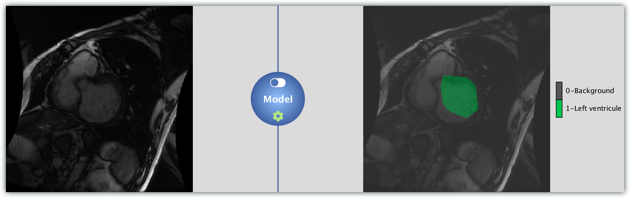
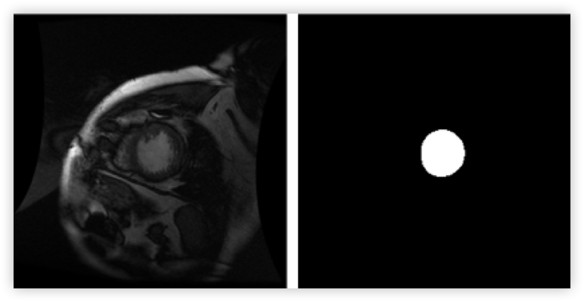
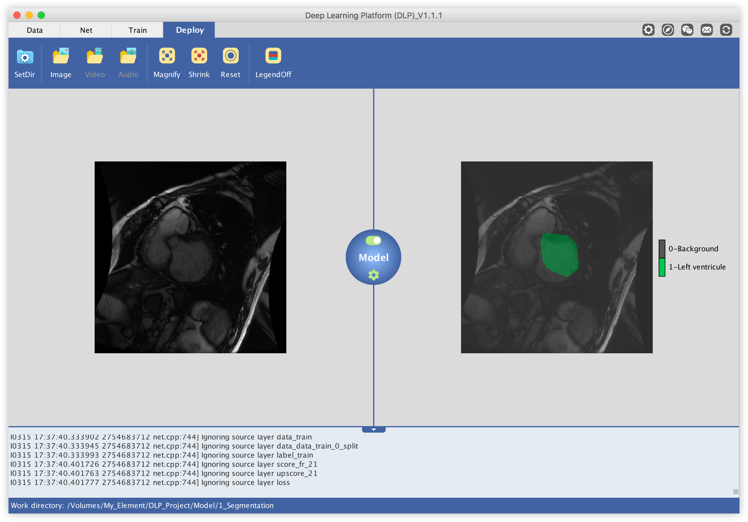
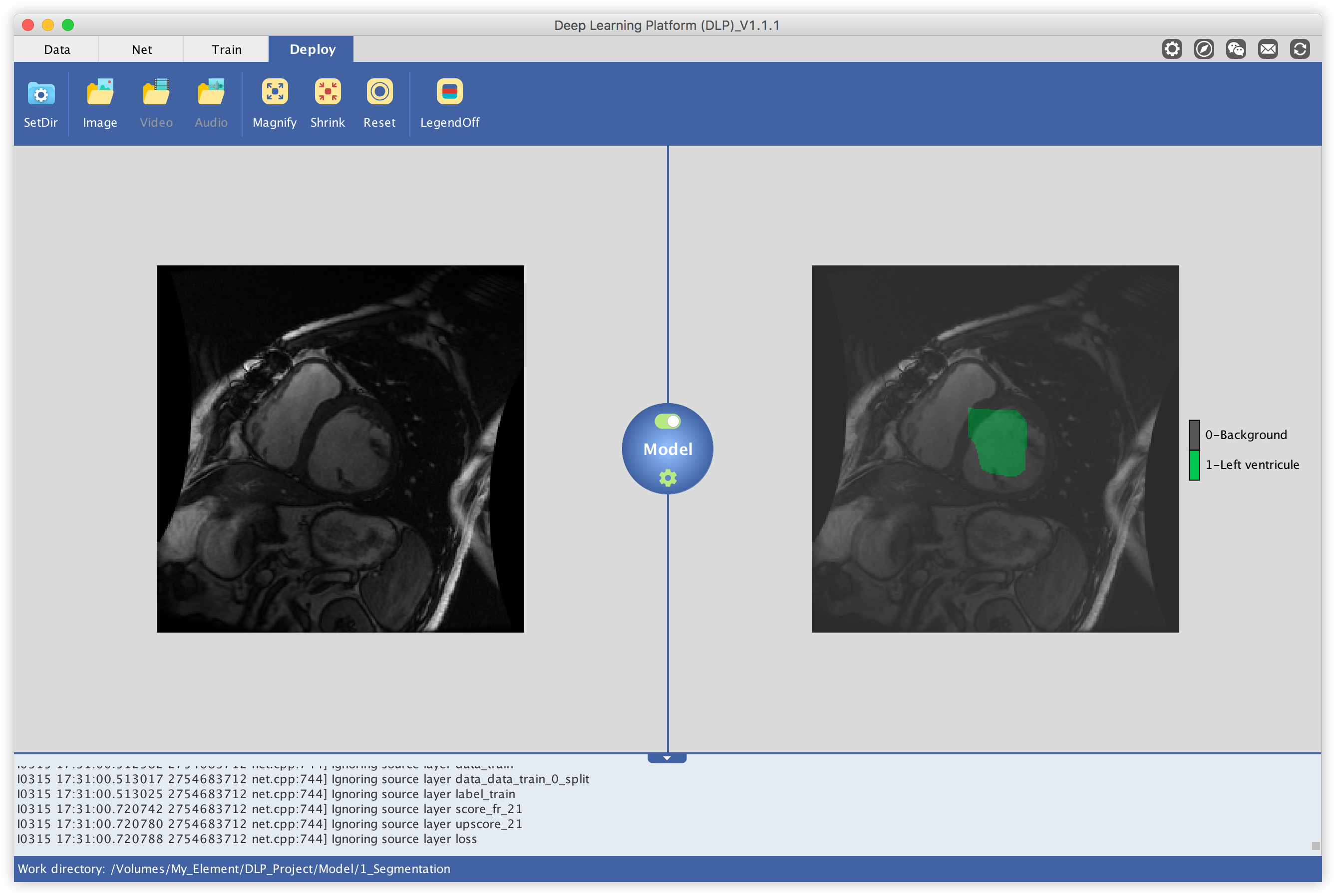
In this tutorial we will see how DLP may be used to train a semantic segmentation network for medical imaging. More specifically, we will use the Sunnybrook Left Ventricle Segmentation Challenge Dataset to train a Caffe model to segment the left ventricle out of MRI images. By the end of this tutorial, you will be able to take a single MRI image, such as the one on the left, and produce a labelled output - outlining the location of the left ventricle in the MRI input image - such as the image in the right.
Set Up DLP
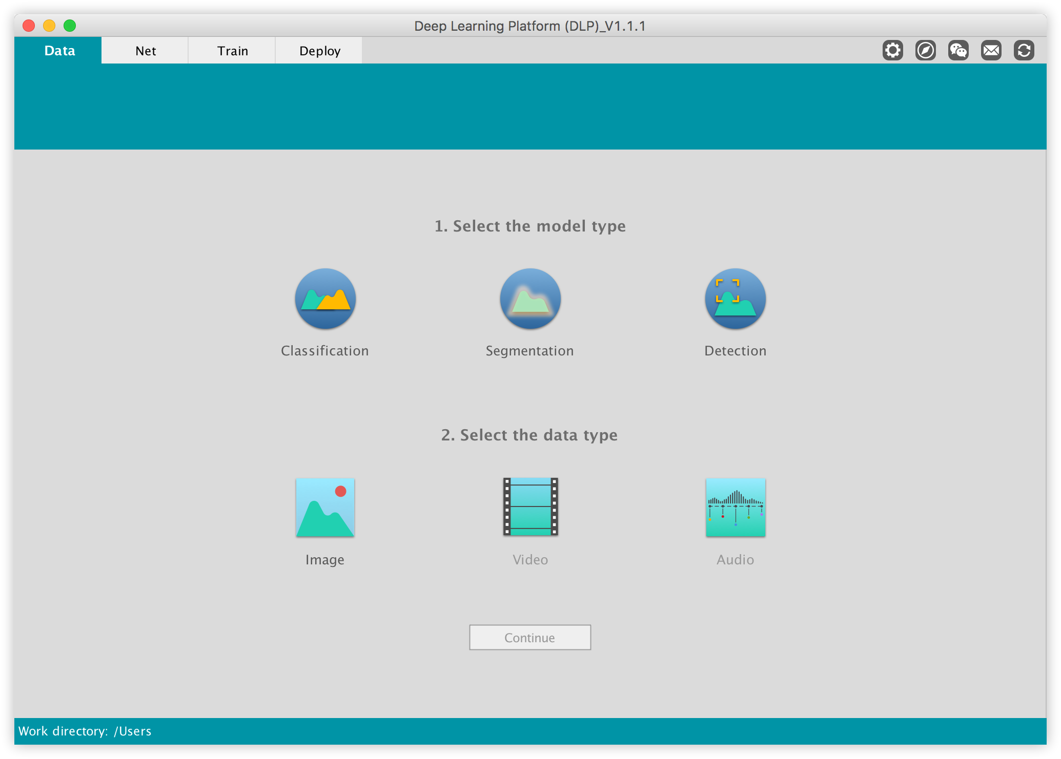
The first step is to launch DLP. If you haven’t installed it yet, you can download it from our website. DLP is built on top of the Caffe deep learning library, so please make sure Caffe is properly configured in your system. Make sure you also compile Caffe's python wrapper. The following window will show up once you launched DLP:
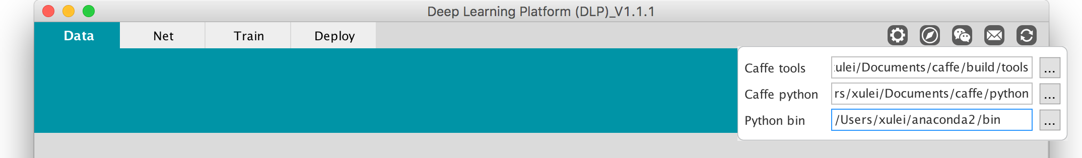
On the upper right corner of the navigation bar, click on the dropdown button. There, specify the paths to Caffe’s tools subdirectory (caffe/build/tools), Caffe’s python wrapper subdirectory (caffe/python), and the path to the bin directory containing your environment’s python (in MacOs and Ubuntu you can enter the “which python” command in your terminal. It will return the path to where python is installed. Python bin should point to that path up to the bin folder which contains Python execution file.).
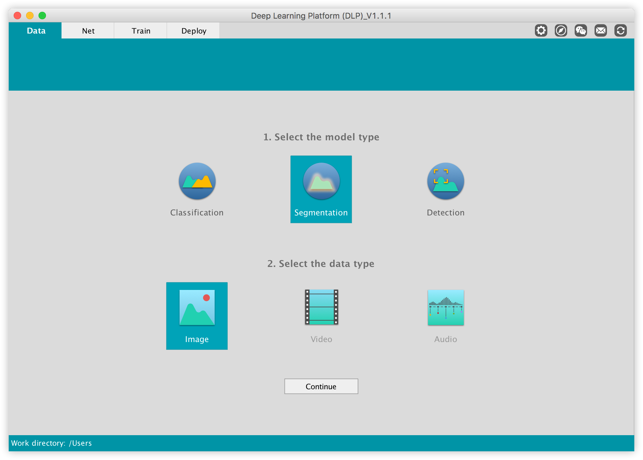
Now under the "1. Select the model type" select Segmentation, and under "2. Select the data type" select Image, then click on Continue.
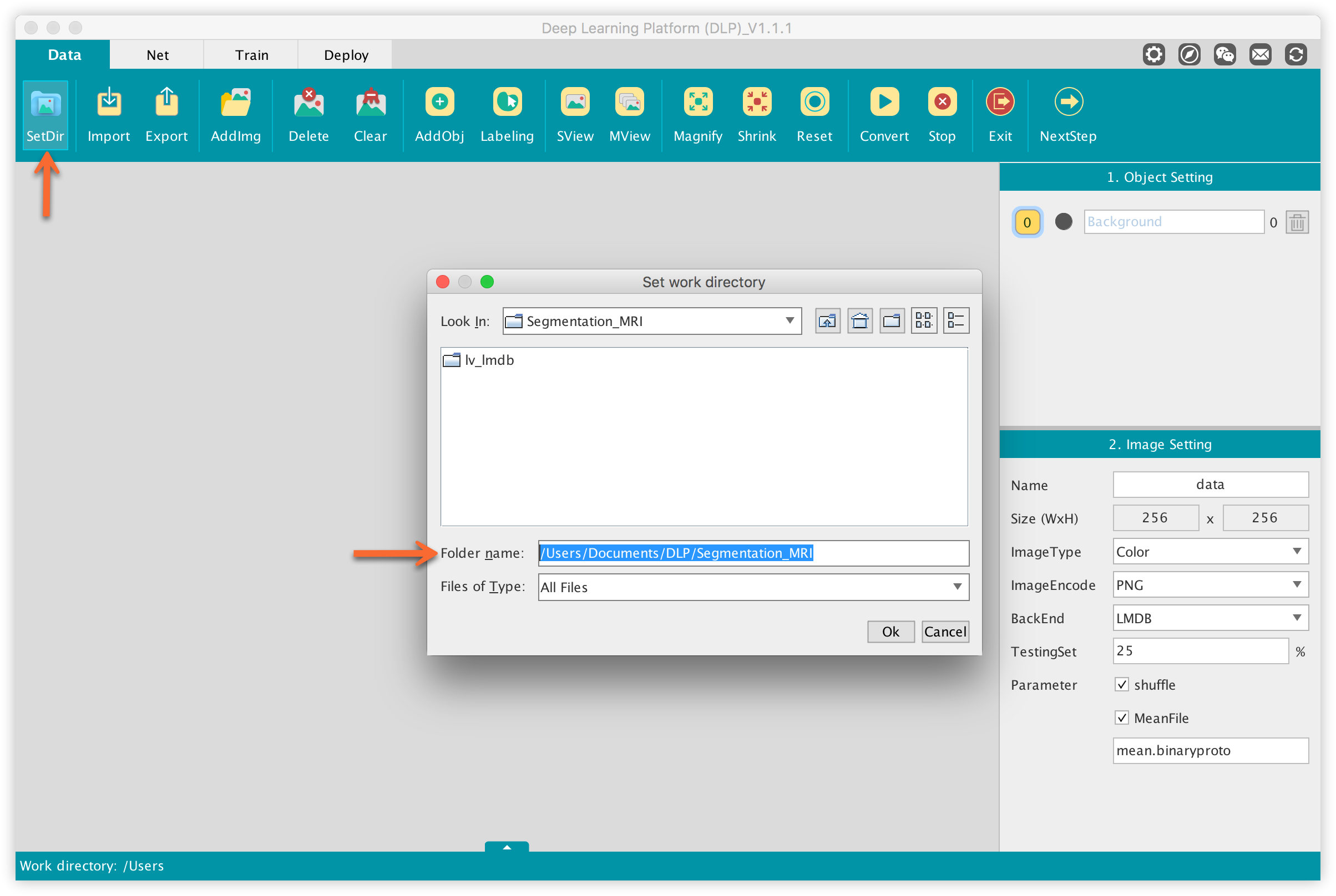
You will land in the window below where the only operation we are going to do will be to set our current working directory. Locate the SetDir button at the upper left corner of the function bar, click on it and a window will pop up where you can set your working directory. Please make sure you specify a file that does not require access permissions. This is important especially for DLP’s Deploy module to work fine.
Get The Dataset
In this tutorial, we will use the Sunnybrook Left Ventricle Segmentation Challenge Dataset. The dataset consists of 16-bit MRI images in DICOM format and expert-drawn contours in text format (coordinates of contour polylines). A sample image/label pair may look like:
You will have to register on the Cardiac MR Left Ventricle Segmentation Challenge website and download links to the dataset will be emailed to you. Unfortunately, in the latest release the filenames have become a little mangled, and don't match up with the contours. For the sake of simplicity, in this tutorial we are going to provide you with the Sunnybrook Left Ventricle Segmentation Challenge Dataset in a format (lmdb in this case) required for Caffe model. Download the data here.
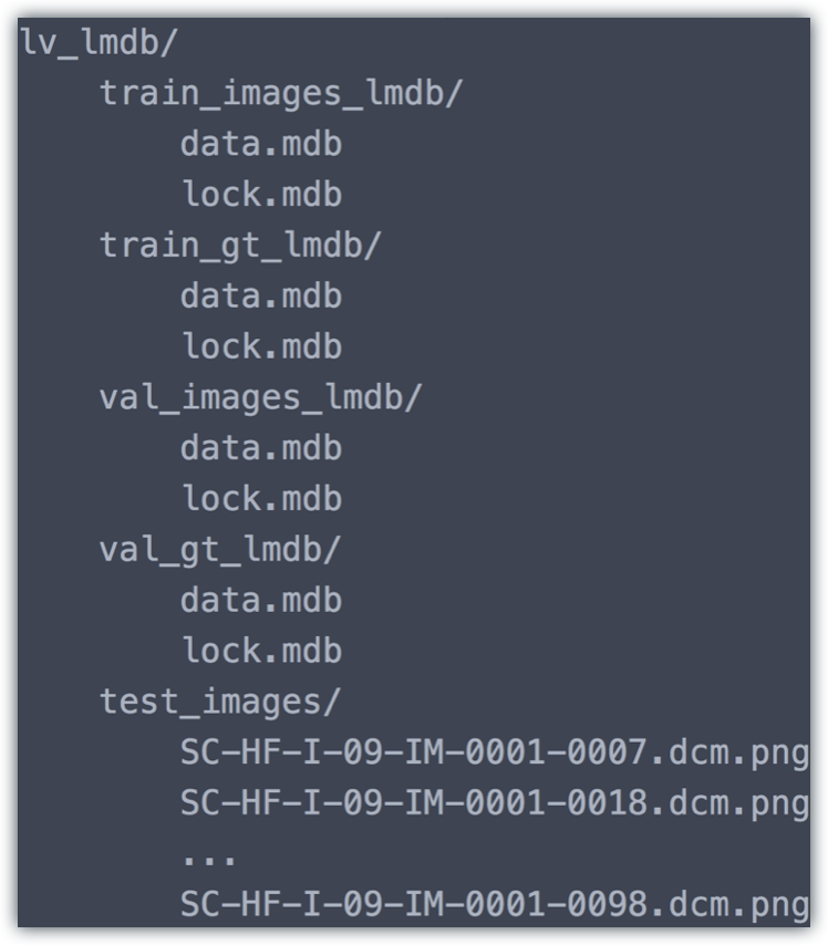
The dataset file structure should look like:
PS: Details on how DLP may be used to generate labels - as the one above - for segmentation task using your own image data will be the subject of an upcoming tutorial.
Model Definition
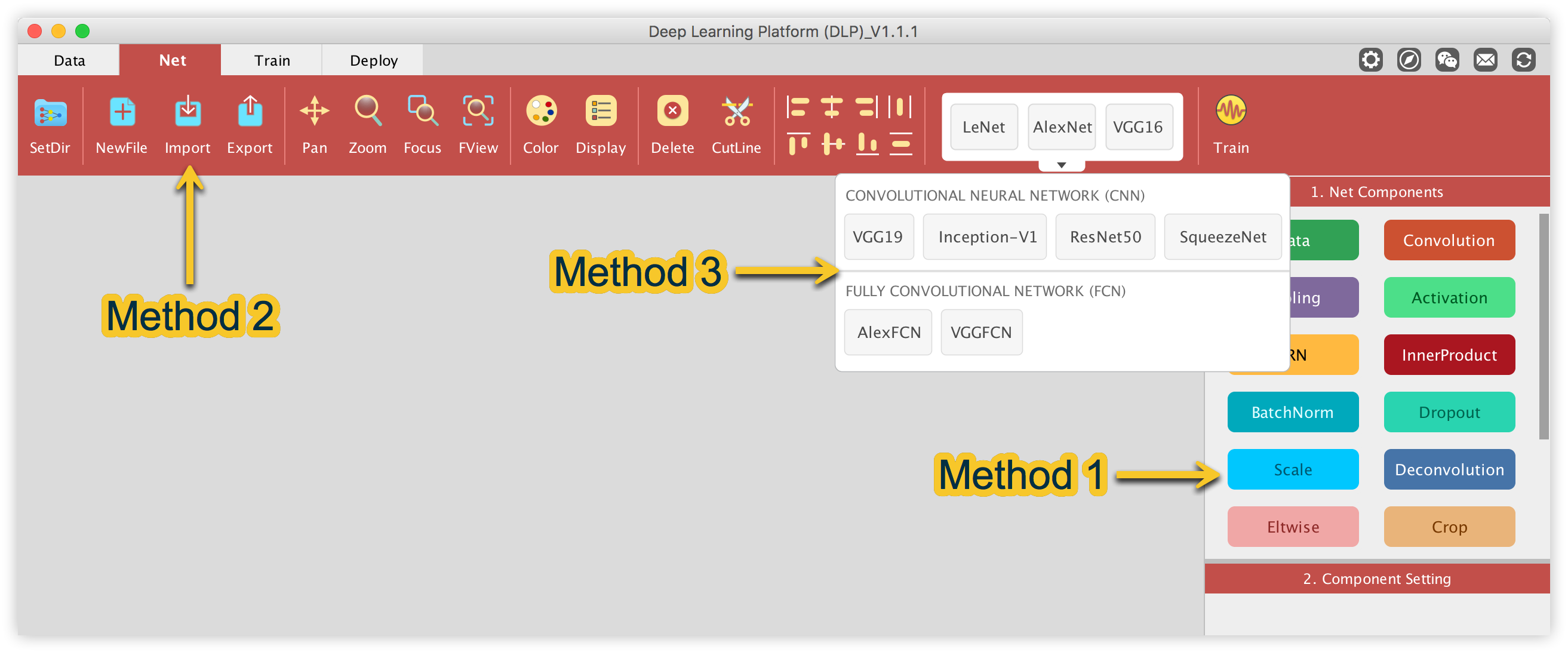
Getting back to DLP, select the Net tab in the navigation bar. This is where we will define our model. There are three ways you can interact with DLP in order to define your network architecture. You can either import your network definition (Caffe ".prototxt" files), build it from within DLP with a drag/drop fashion using DLP’s Net Components, or simply select one network architecture from the list of predefined network architectures present in DLP’s Net Library.
In a past tutorial, we introduced DLP and how it may be used to Train a convolutional neural network (CNN) classifier. We defined image classification as the task of classifying what appears in an image into one out of a set of predefined classes. This assumes that there is only one object of interest/focus in the image.
Image segmentation is a much more sophisticated task. Given an image, its goal is to divide the image into segments/regions belonging to the same part/object/content. One way to achieve that is to use a technique known as image semantic segmentation.
Image semantic segmentation can be thought as a generalization of image classification. Given an image, its task is to classify every single pixel in the image into one out of a set of predefined classes. Such a image classification tends to create contours around part of the image because nearby pixels are often of the same class and hence, is a technique used for image segmentation.
Now a fully convolutional network (FCN) is one where all the learnable layers are convolutional, so it doesn’t have any fully-connected layer. This is to contrast with CNN which has some convolutional layers followed by one or a few fully-connected layers. The idea is to preserve the spatial arrangement from the input image which is useful for image segmentation.
In order to train an FCN for semantic segmentation, a suitable pre-trained classification model (trained on the ImageNet classification dataset) must be used. Basically, standard pre-trained classification networks (such as AlexNet, and VGGNet) are converted into fully convolutional networks and their learned representations are transferred by fine-tuning to the semantic segmentation task. Converting a standard CNN to FCN (also known as convolutionalizing a CNN) is usually a three-step process:
1. Start with a pre-trained CNN for classification, i.e: AlexNet
2. Convert all the fully-connected layers to convolutional layers with 1x1 filter/kernel size.
3. Add a deconvolution (or transposed convolution) layer(s) on top of your network to scale up, the scale down effect made on previous layers. The idea is to recover the activation positions to something meaningful related to the size of the image.
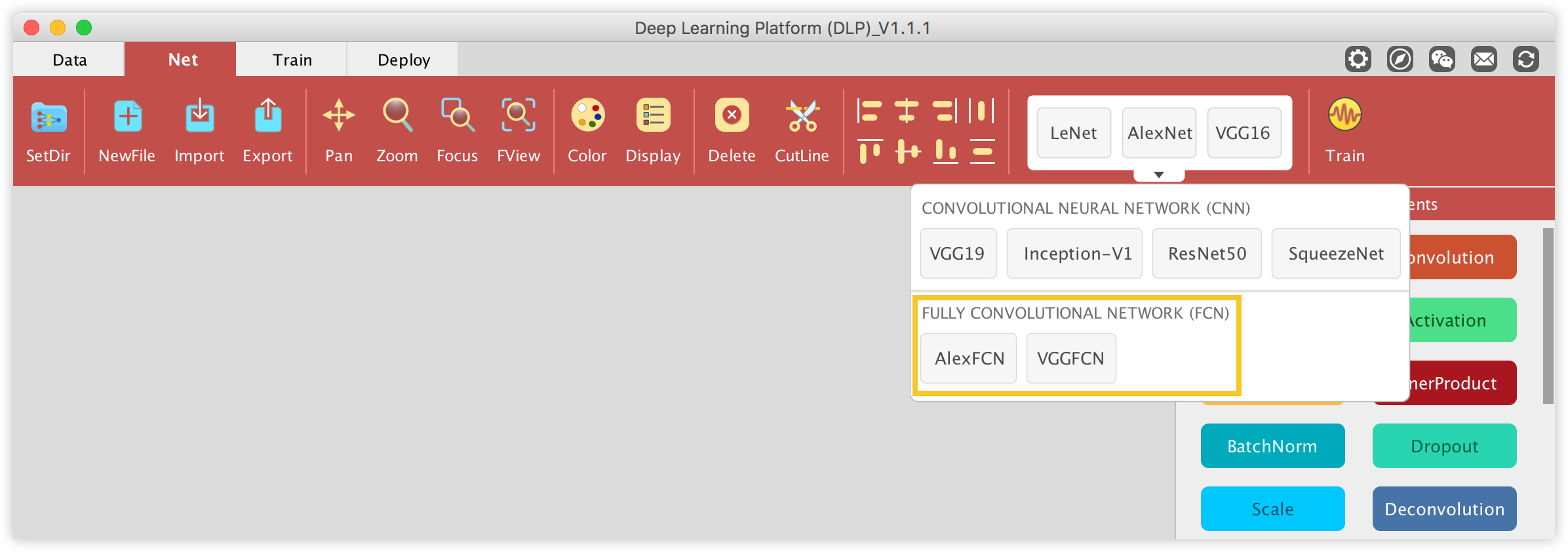
In the DLP Net Library, two FCN architectures from fcn.berkeleyvision.org are available.
We will use AlexFCN. In order to successfully train AlexFCN, we will need the convolutionalized (converted from CNN to FCN) pre-trained AlexNet model which can be downloaded from here. Now drag the AlexFCN button from the Net Library and drop it into the visualization area.
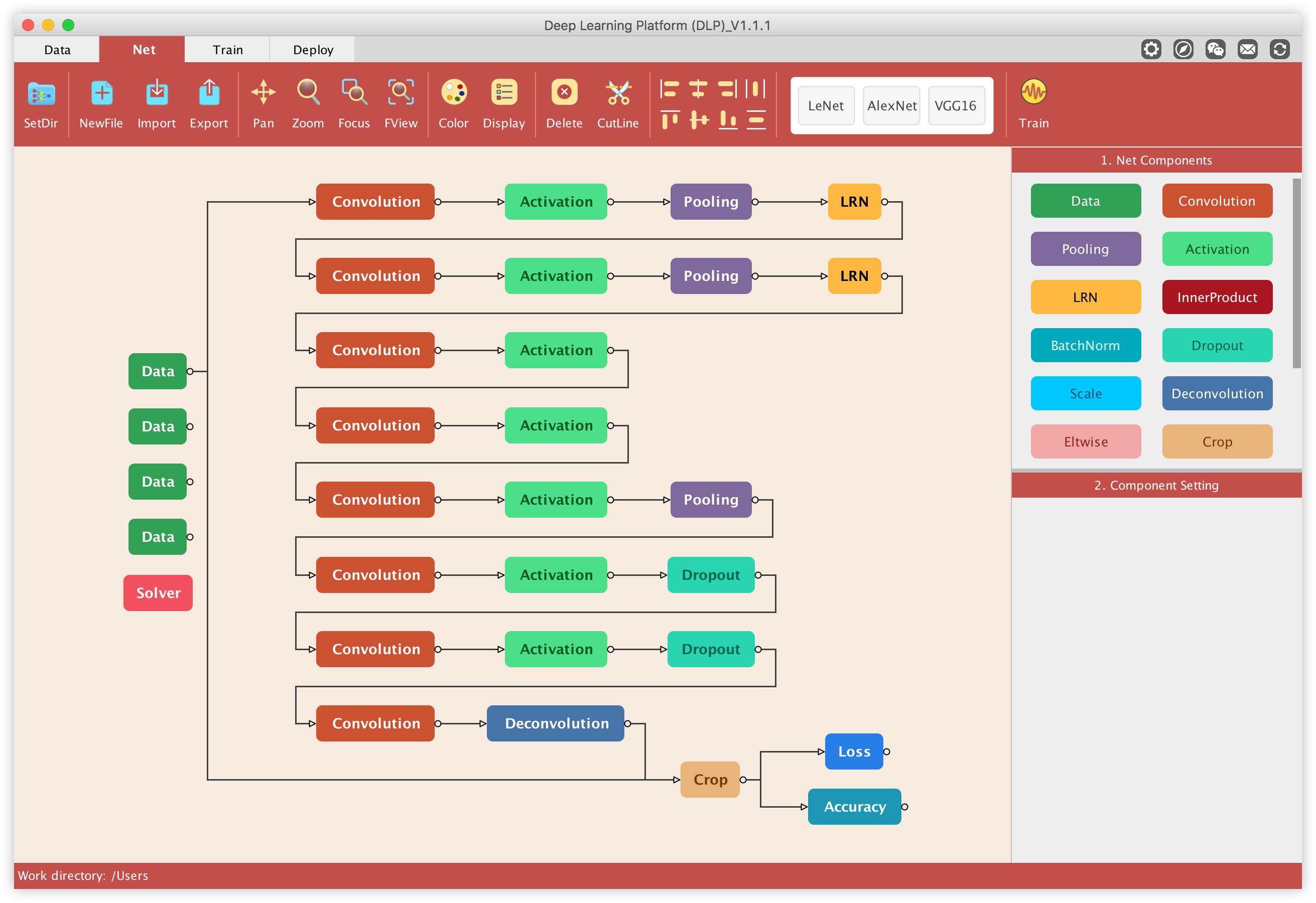
Now we need to define/modify the network architecture to fit our semantic segmentation task which is to segment the left ventricle out of MRI images.
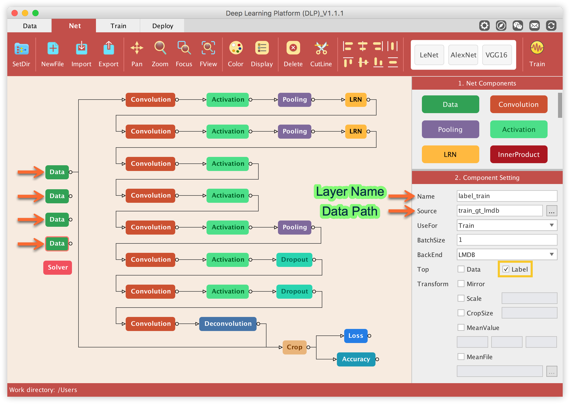
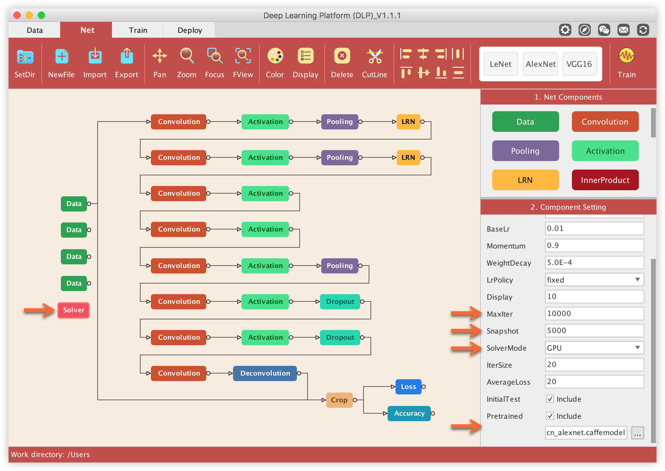
First off, we need to feed the data into the network. This is done by clicking on the Data component/layer of the network and in the Component Setting panel, set the path to the lmdb file corresponding to that Data layer. In order to know which lmdb file goes to which Data layer, refer to the default name given to each data layer (you can edit those names but it is recommended not to). For instance in the image below, the Name property (in the Component Setting) associated to the highlighted Data layer is label_train. This means that the Source property must point to the lmdb folder referring to the labels of the training data, which is named train_gt_lmdb in the dataset.
Do the same for all the other Data layers, each time paying attention to the Name property of each Data layer to figure out what lmdb file should go where.
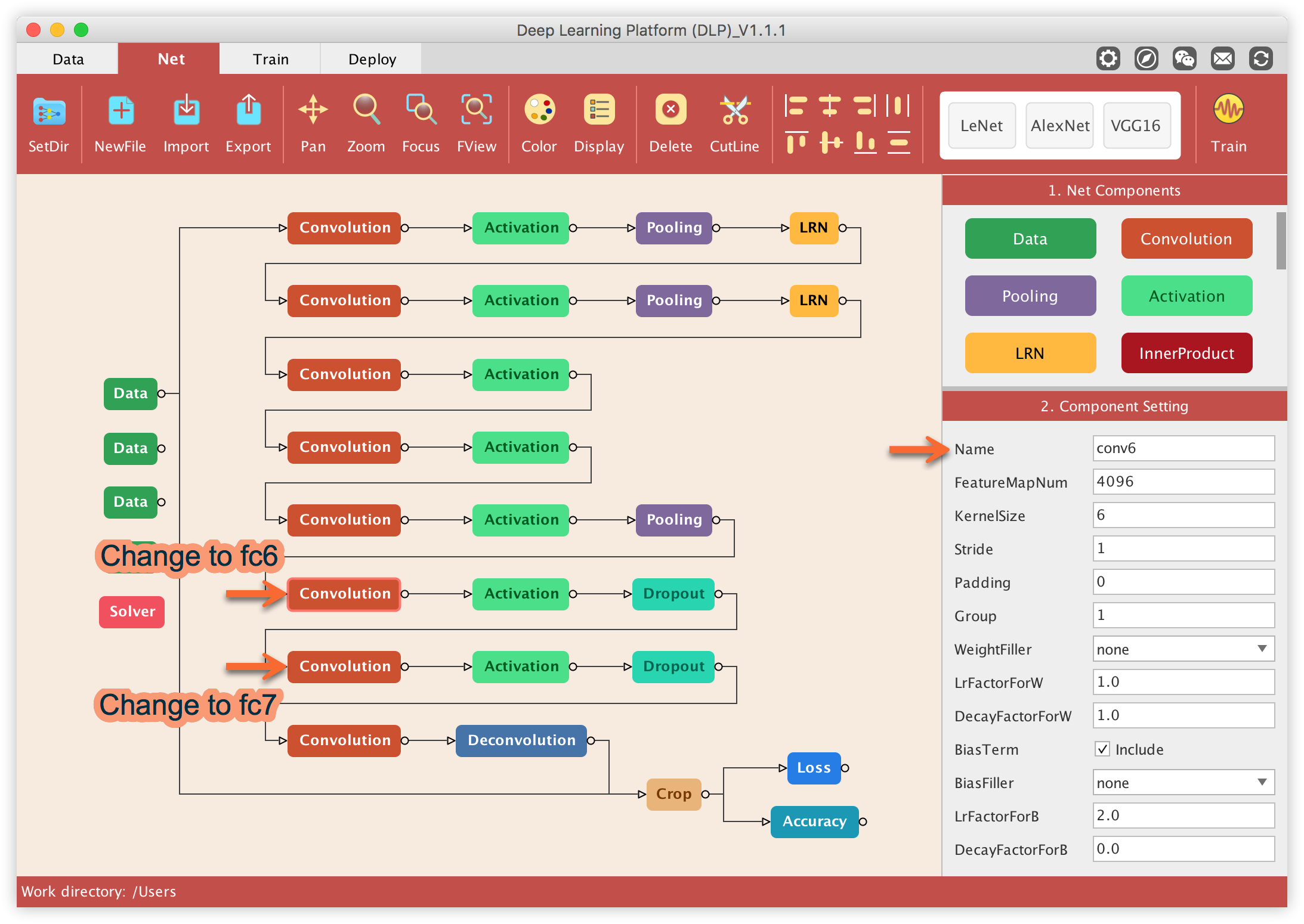
Next, we want to modify the Name property associated to two convolution layers in our network. More precisely, we want to change convolution layers associated to the Name conv6 and conv7 to fc6 and fc7, respectively. This is to make sure that all the layers name in our network matches the layers name from the pre-trained model (AlexNet in this case) which will define shortly. This is important for transfers learning and fine-tuning which are required to successfully train our model.
Next, make sure the FeatureMapNum property of both the last convolution layer and the deconvolution layer, is set to 2. This is because our segmentation task has only one object of interest (the left ventricle) in any given MRI image. So the pixels associated to the left ventricle were set to 1 and everything else (background) set to zero, which boils down to a 2-class classification task. We should keep in mind that semantics segmentation learn to predict pixel-wise classification. So for this network, the FeatureMapNum property of both the last convolution layer and the deconvolution layer should be set to “the number of object of interest in your dataset + 1”.
Lastly, we should define/modify some properties of the Solver component. We want to train this model for a maximum of 10k iterations and save a snapshot every 5k iterations. We can either train on GPU or CPU and this is defined by the Solver Mode property. Last but not the least we need to specify the pre-trained model which we downloaded above, and this is done under the Pretrained property of the Solver component.
We are now up and ready to launch the training via the Train button which is located at the right of the Net Library. Clicking on the Train button will trigger a pop up window requiring you to save your network structure information, and will direct you to the Train module.
Model Training
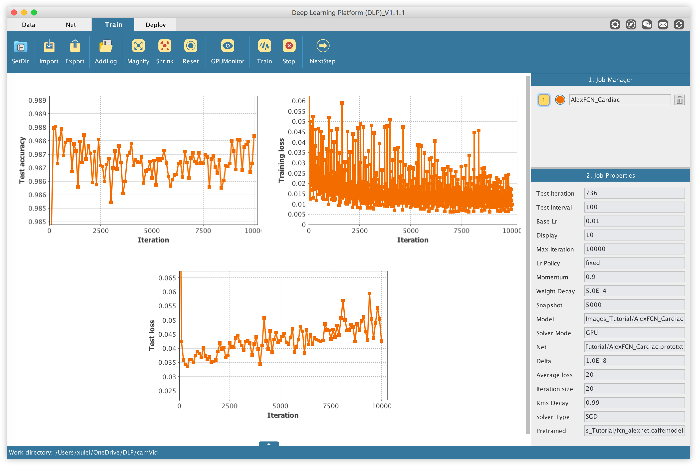
The Train module is where the training takes place, which can be monitored via different plots.
Notice that the accuracy score on the validation data starts very high (a little bit over 98%). This is understandable given that less than 2% of pixels of each MRI image represent the left ventricle. So it suffices for the network to classify every single pixel as background for it to reach such a high accuracy. This is the reason we have to train the model for longer, to make sure it actually learns the intrinsic features of the data in order to perform well rather than just lazily classify all pixels as background.
Once the training is completed, a pop up message will notify of the completion. Click on ok, and on the NextStep button to land in the Deploy tab.
Model Inference
Click on the NextStep command to head to the Deploy module.
If you have followed this tutorial correctly, you would be able to use your trained model to make inference on unseen MRI image data. We are going to use MRI images located under the subdirectory test_images from the dataset we downloaded previously. These images are a subset of the test set from the Sunnybrook Left Ventricle Segmentation Challenge Dataset.
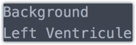
To start making predictions on new image data, there are two files we need to prepare: a deploy.prototxt file, and a text label file. Your label.txt file should contain the following:
where the background Indicates everything that is not a left ventricle.
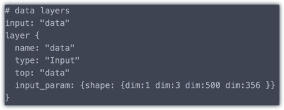
To create the deploy.prototxt file is quite straightforward as well. Remember at the end of the Model Definition section you were prompted to save your model structure under Caffe ".prototxt" file format. Open up that file and copy everything from there except for the data layers, loss layer, and accuracy layer. Create a deploy.prototxt file and paste there. Then at the very top or beginning of the file, insert the following:
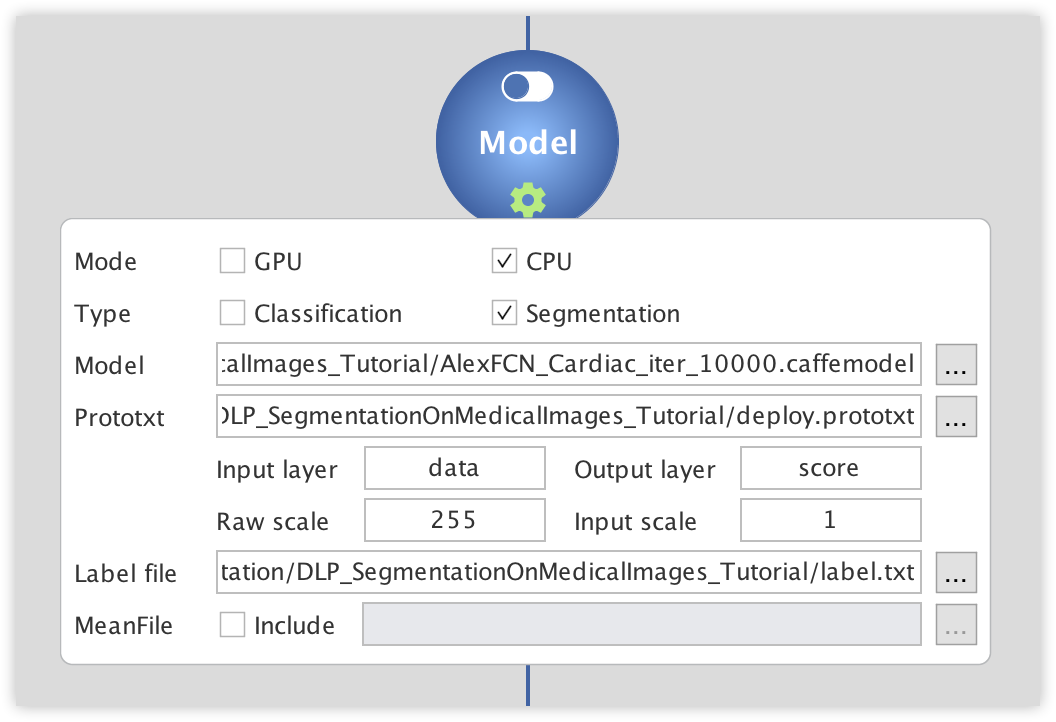
Next click on the dropdown button to configure the inference engine. There we will specify whether or not to use GPU during inference, the type of inference to perform, and set up paths to the caffemodel we just trained and to the deploy.prototxt and the label.txt we created jut above.
The dropdown button will turn green signaling that all required parameters have been provided. Then turn on the toggle button to start the inference engine.
Now all what remains to do is to load an image like the one on the left, and the model will output the same image but with the predicted location of the left ventricle highlighted like the image in the right.
The predicted results will be saved as images in the designated folder.
Conclusion
We'd love to hear about your experience using DLP, or if you have any further questions, or just want to discuss any issues you experience with the tutorial, please get in touch via our official email account [email protected].