Multi-Class Classification Using DLP With Keras As Backend

DLP, which stands for Deep Learning Platform, is a piece of software for AI application development and currently wraps two deep learning frameworks: Caffe and Keras. DLP aims to allow developers to focus on network architecture design without having to deal with the overhead that may come with the actual implementation of designing, training, and testing a deep learning model.

In this tutorial, we will walk you through the process of developing and evaluating a deep learning (DL) model for multi-class classification problems using DLP with Keras as backend. After completing this step-by-step tutorial, you will know:

1. How to prepare dataset for classification problems in DLP’s Data module

2. How to design your own network architecture or make use of existing architectures available in DLP's network library

3. How to train your neural network in DLP’s Train module

4. How to perform batch inference on unseen dataset using your trained model in DLP’s Deploy module

1. Environment Setting

In this tutorial, we will use DLP with Keras as the backend. Therefore, naturally we should have Keras installed in our system or virtual environment.

DLP has been tested on Mac, and Ubuntu with Keras 2.2.4 and Tensorflow backend. You can install Tensorflow by typing the following commands in your terminal:

$ pip install tensorflow

or:

$ pip install tensorflow-gpu

for NVIDIA GPU support.

Keras can be installed by typing the following command:

$ pip install keras==2.2.4

You can check whether Keras with Tensorflow as backend is working properly by running the following command in your terminal:

$ python -c 'import keras’

That command line should return Using TensorFlow backend, if Keras is configured properly for a Tensorflow backend.

Then head to DLP website to download its latest version.

2. Problem Description

In this tutorial, we will train a neural network model on the Fashion MNIST dataset to classify images of clothing, like sneakers and shirts. Fashion MNIST contains images of various articles and clothing items - such as shirts, shoes, bags, coats and other fashion items - consisting of a training set of 60,000 examples and a test set of 10,000 examples. Similar to MNIST, each example is a 28x28 grayscale image associated with a label from 10 classes (top, trouser, pullover, dress, coat, sandal, shirt, sneaker, bag, and ankle boot).

You can download the dataset from here: fashion_mnist_data.tar.gz. The fashion_mnist_data.tar.gz file has the following directory structure:

<training/testing> / <label> / <id>.png

3. Configure DLP for Keras backend

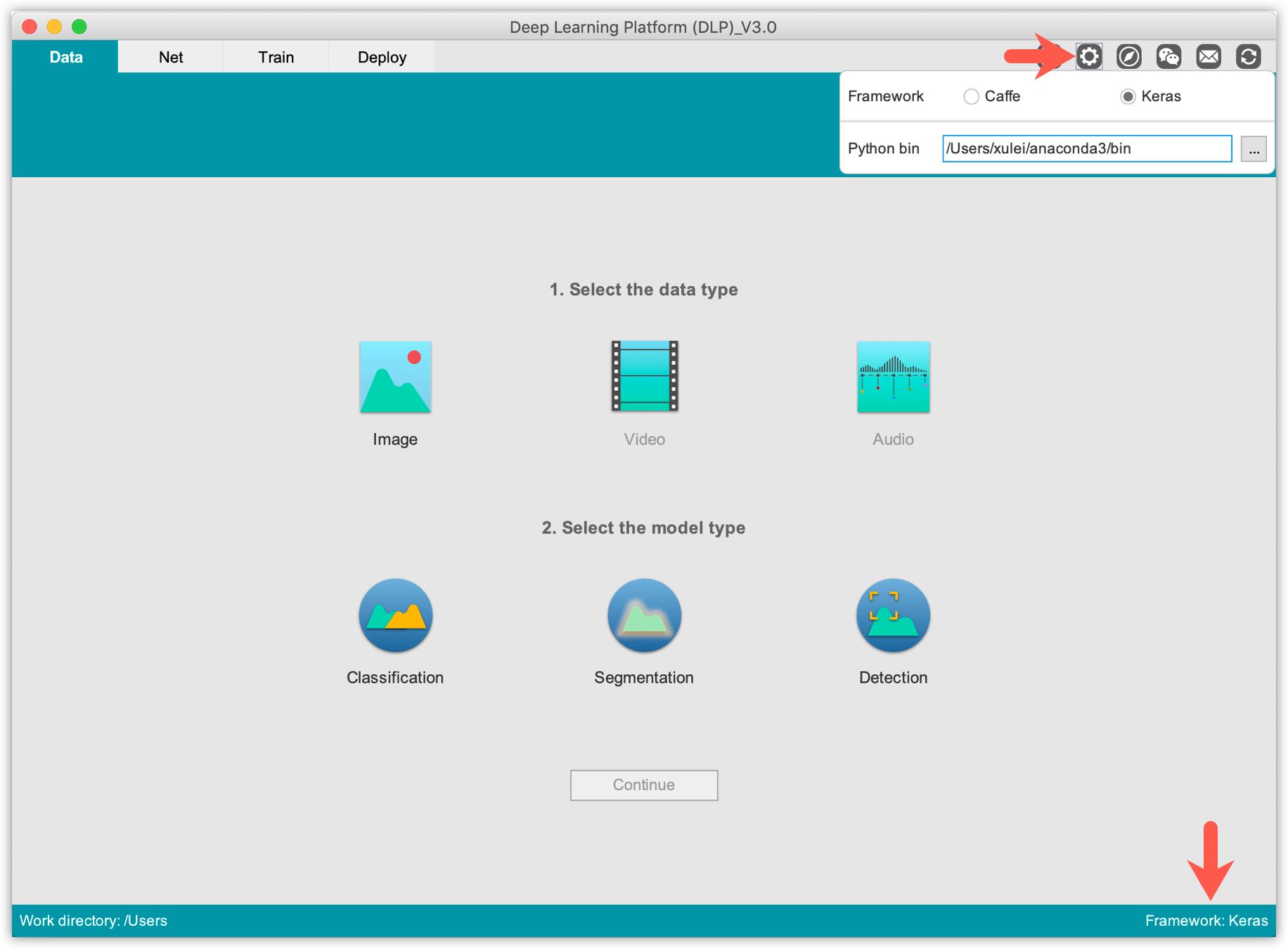
Assuming you have installed the latest version of DLP (get it here), open it up. The first action we have to do is to configure DLP for Keras backend. This is done by selecting the Keras option under the setting button located on the menu bar at the top right. Once you have selected Keras, you will have to specify the bin path to your python environment. This is the environment where you have installed Keras and Tensorflow. You can locate it with the following command:

$ which python

There is an indicator at the bottom right of the window, which specifies the framework DLP is currently configured for. It should now read Keras.

For a classification task, under the 1. Select the data type select Image, then select Classification under 2. Select the model.

Click Continue to move to the Data module.

4. Prepare the Dataset

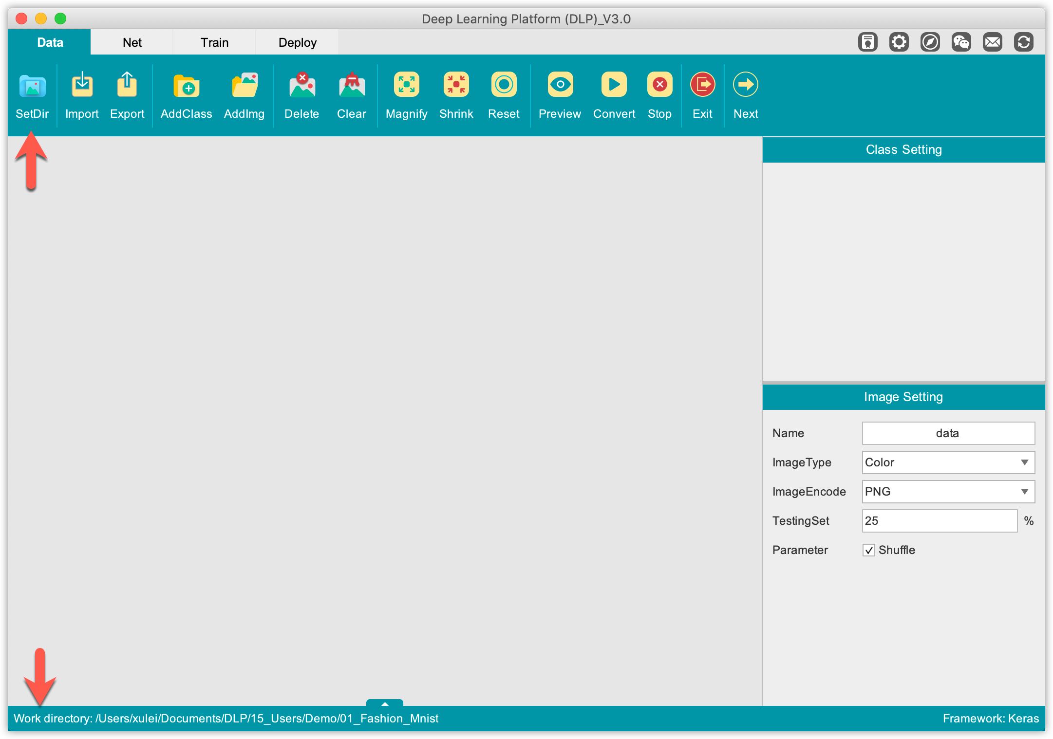
Before getting to load and prepare your image dataset for training and validation, it is good practice to first set up a working directory for your project. You do it by clicking on the SetDir button at the top left corner on the functions bar, then select (or create) the working directory for the project. Additionally, there is an indicator at the bottom left corner of the window that indicates your current working directory.

Loading your images in DLP is a two-step process:

1. Add the class label (internal class index starting from 0).

2. For each class label, add the corresponding images.

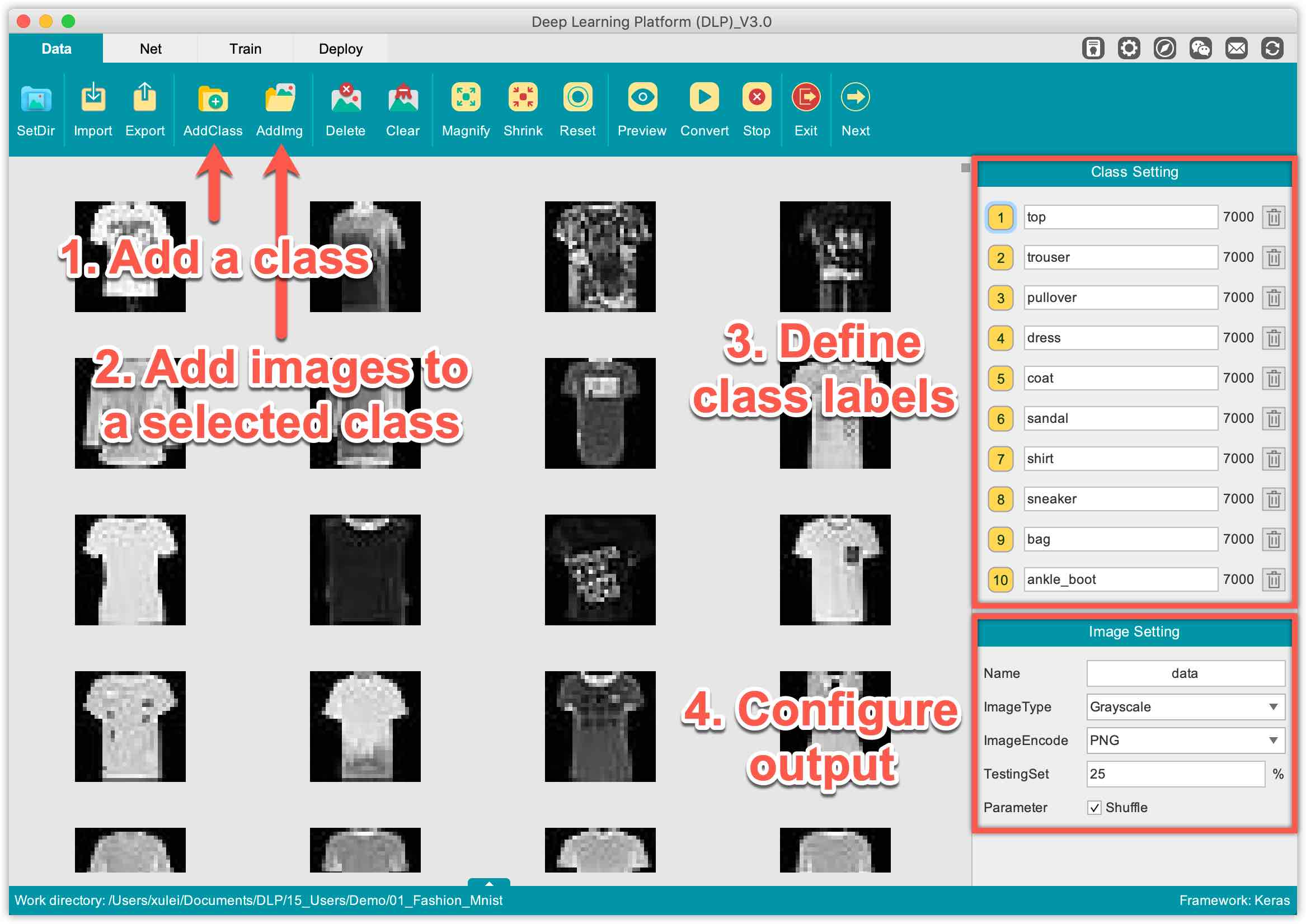
The Fashion MNIST is a 10-class classification problem. So we are going to add 10 class labels. To add a class label, under the functions bar click on the AddClass button. Then specify the label for the class. For the first class, the label is "top", for the last class, the label is "ankle_boot", and etc.

To add images corresponding to a class label, first click on the numbered-yellow box associated with it on the Class Setting panel, click on AddImg and navigate to the folder containing the images associated with the class label. It may happen that you associated some images to the wrong class label or that some class labels are associated to the same images. To correct that, you can delete all images associated to a class label simply by clicking on the yellow box associated with the class label to inspect the images, then click on the Clear button on the top function panel to delete all images.

Once you have added images for each class, what remains to do before building the dataset is to specify dataset configuration such as the train/validation split ratio, the image type (grayscale or RGB), the encoding type (.png or .jpg), etc. It doesn’t matter whether the images you loaded from your local disk into DLP are grayscale or RGB color, because you can always change their type by specifying the image type you want based on your application. For instance, Fashion MNIST is a dataset of grayscale images but by specifying Color for image type, DLP will convert the grayscale images into RGB images.

You can now click on the Convert or Export button, located on the top function panel, to process the dataset based on your image settings. It is important to note that during this data preparation stage, we do not have to worry about the shape of our images (i.e., images can be of different/any shapes). This will be taken care of on the next stage, network definition, during the configuration of the neural network model.

5. Define the Neural Network

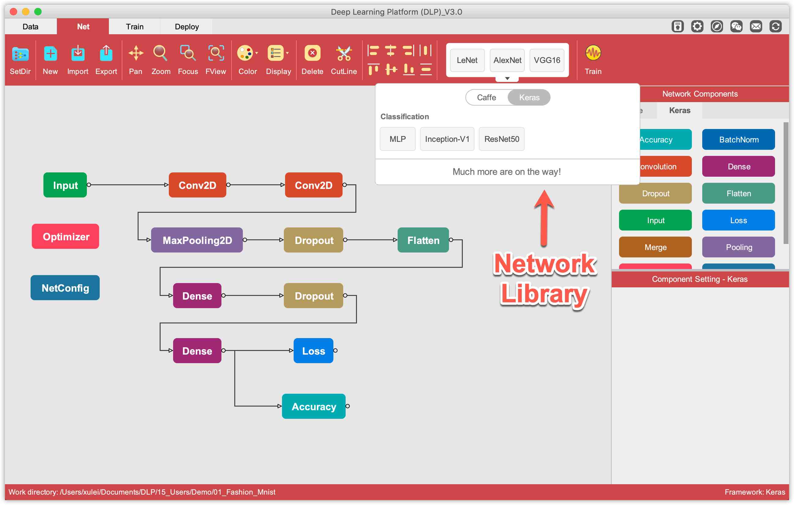
DLP offers a visual interface to make it easier to define and build your neural network. You can either define your own neural network from scratch or use one of the pre-defined popular architecture available in DLP’s Net library under the Net tab window.

Defining a neural network with DLP boils down to connecting the different network components (layers) to each other. Roughly speaking, a DLP network should be composed of the following elements:

1. Input layer: which should be connected to the first layer of the neural network. This is where we define, among other thing, the dataset source (either from Keras built-in datasets or from local disk), the desired shape of our image dataset (by specify the height, the width and the channel parameters), etc.

2. Hidden and output layers: typically composed of layers such as convolutions, pooling, batch normalization, dense, etc. connected to each other. This is where you define the hidden layers and output layer of your architecture.

3. Loss layer: which should be connected to the output layer (last layer) of your architecture. This is where you define the objective function to be minimized during network training.

4. Accuracy layer: which should be connected to the output layer of your architecture. This is where you define the function to be used to evaluate your model during training.

5. Optimizer: it’s a standalone layer/component where you specify the parameters of the solver, i.e. defining the optimization algorithm to be used and configuring its parameters.

6. NetConfig: which gives you more control over monitoring the training process. This is also where you select whether to use a CPU or GPU for training. This layer is a standalone component.

In this tutorial, instead of building a network architecture from scratch (simply by dragging elements of your architecture from the Network Components panel, dropping them into the workspace, and connecting them together), we will use one of the pre-built neural network architecture made available via DLP’s network library. Typically the network we are going to use is the LeNet architecture. Head to the net library then drag and drop the network named LeNet into the workspace.

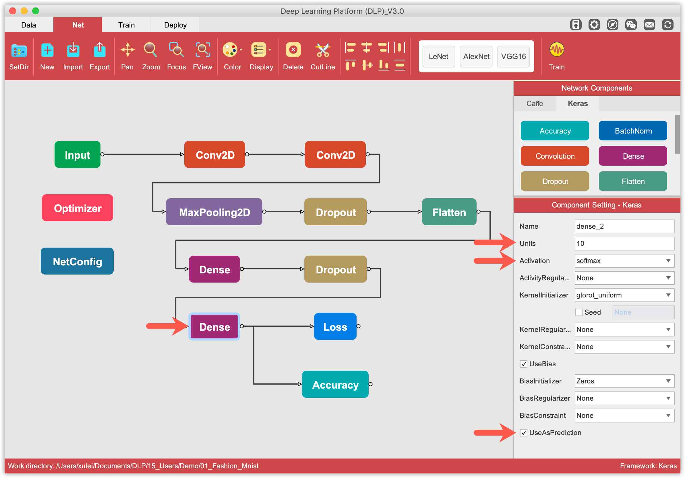
The input layer: firstly specify the source of our dataset, and the shape we’d like to give to that dataset. Since we have prepared our own dataset, we specify Local disk for the Source parameter. This implies that we have to specify paths to the training set and validation set, of our dataset. Next, we need to define the shape of our dataset. The input to our network should be of shape (batch_size, height, width, channel). Since our images data are grayscale, the channel must be set to 1. The other three parameters are defined empirically. Though Fashion MNIST is composed of images of resolution 28x28, we are going to reshape them to 96x96 so we can train our model on images of resolution 56x56.

The hidden layers and output layer: here we are mainly concerned about the output layer, which number of units/nodes should match the number of class labels in our dataset. Since our dataset has 10 class labels, therefore the output layer Units parameter should be set to 10. The Activation in this layer (the output layer) should be set to Softmax since we are dealing with a multi-class classification problem. There are multiple other parameters both in hidden and output layers, which you can play with. For instance you can decrease or increase the dropout rate defined in the Dropout layer. Lastly, an important parameter common to every layers — other than the input, the loss, the accuracy, the optimizer, and the NetConfig layers — is the UseAsPrediction parameter. This is the parameter that tells DLP which of your layer(s) is (are) output layer(s).

The optimizer layer: we are going to use the default values for this layer. That is, we are going to train our neural network for 2 epochs, using stochastic gradient descent (SGD) with momentum and learning rate decay.

The NetConfig layer: we are going to use the default values for this layer. That is, we are going to monitor the accuracy of the model on the validation set every 1 epoch and only save the best model.

Once all layers are configured properly, click on the Train button on the Function Bar to save your network architecture on local disk (.prototxt), and to launch the training process.

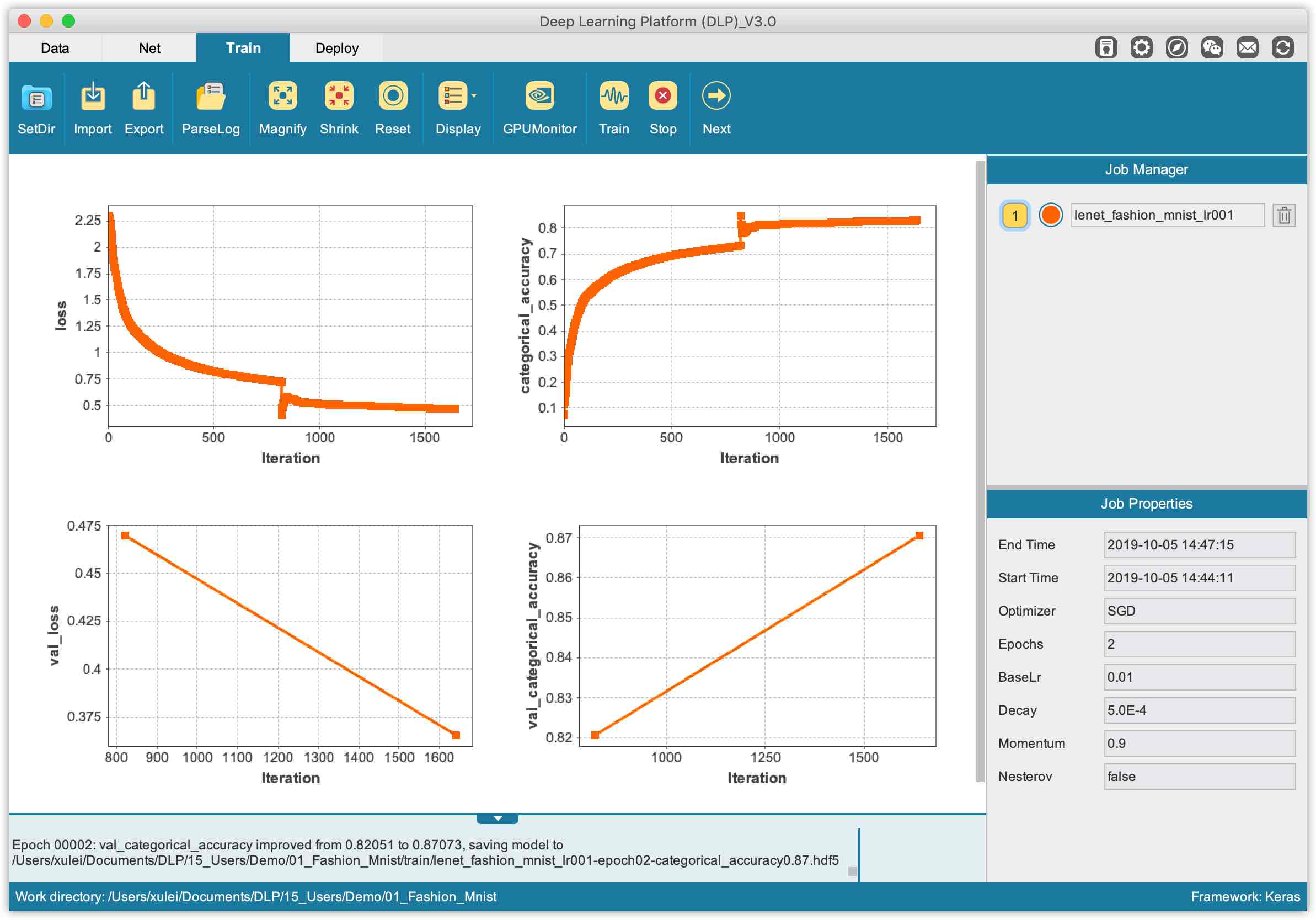
6. Monitor the Training

You can now visually monitor the training via various plots of training/validation loss and accuracy at each batch iteration. For instance, we can read that after the first epoch the accuracy of the model on the train set clocks around 86% while the accuracy on the validation set is above 87%. Keras models are .h5 or .hdf5 files. These files will be saved in the same directory you specify when you clicked the Train button and saved details of your network architecture.

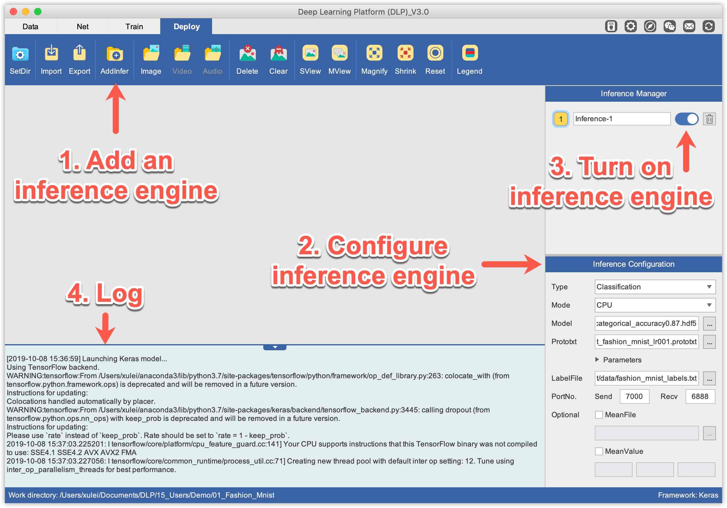
7. Model Inference

You can now test your model on unseen samples. Head to the Deploy tab, and add an inference engine by clicking the AddInfer button on the function panel. Once an inference engine is added, you can configure it in the panel located at the lower right of the Deploy tab window.

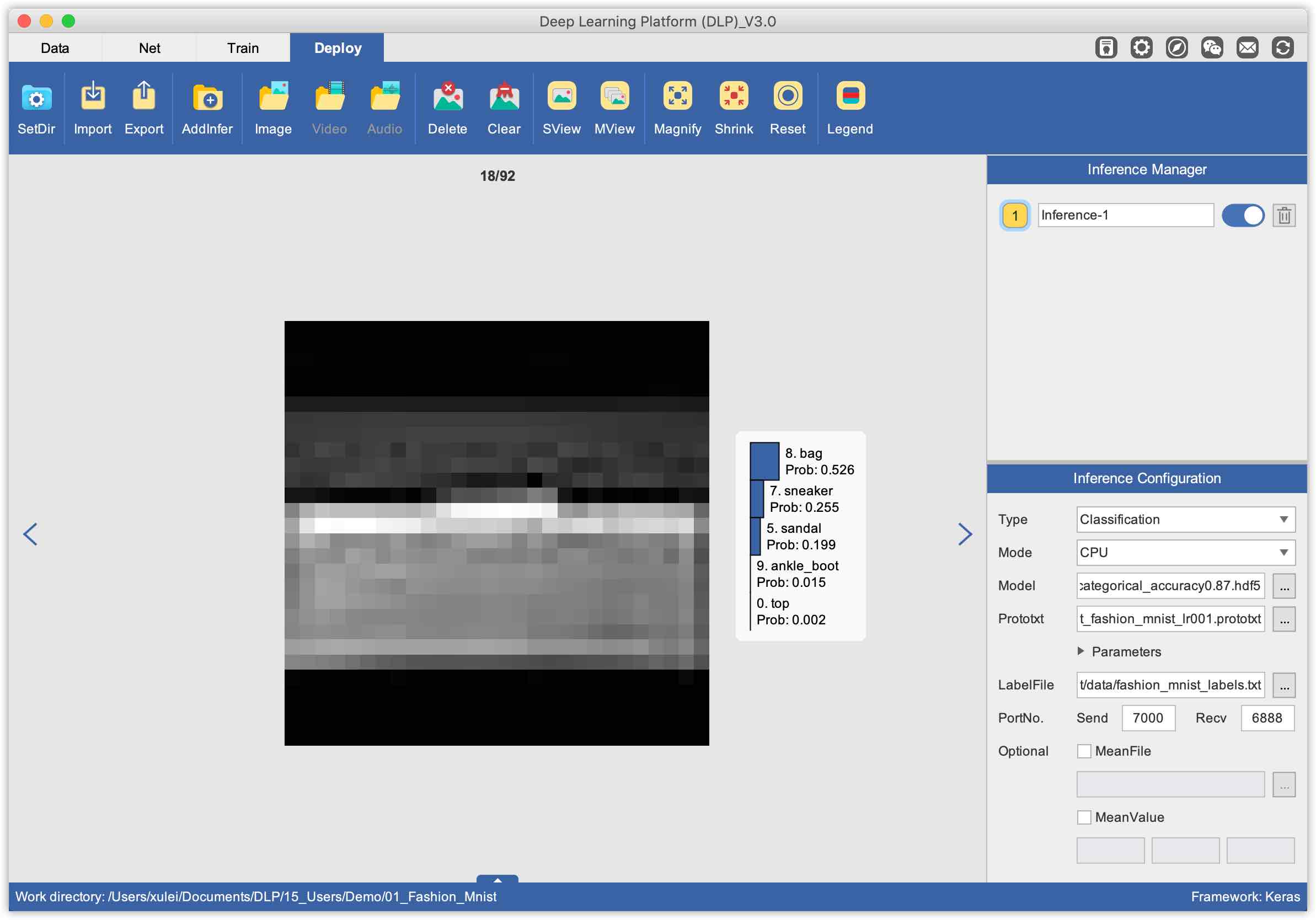
Now we are all set to configure the inference engine. Typically, we have to define the type of inference we want our engine to be ready for, load the trained model via the Model parameter, load the network architecture via the Prototxt parameter, load the label file text via the LabelFile parameter, and eventually edit the inference engine port number — via the PortNo. parameter — just in case the defaults are already in use. Then, turn on the inference engine by clicking the switch beside the inference engine name.

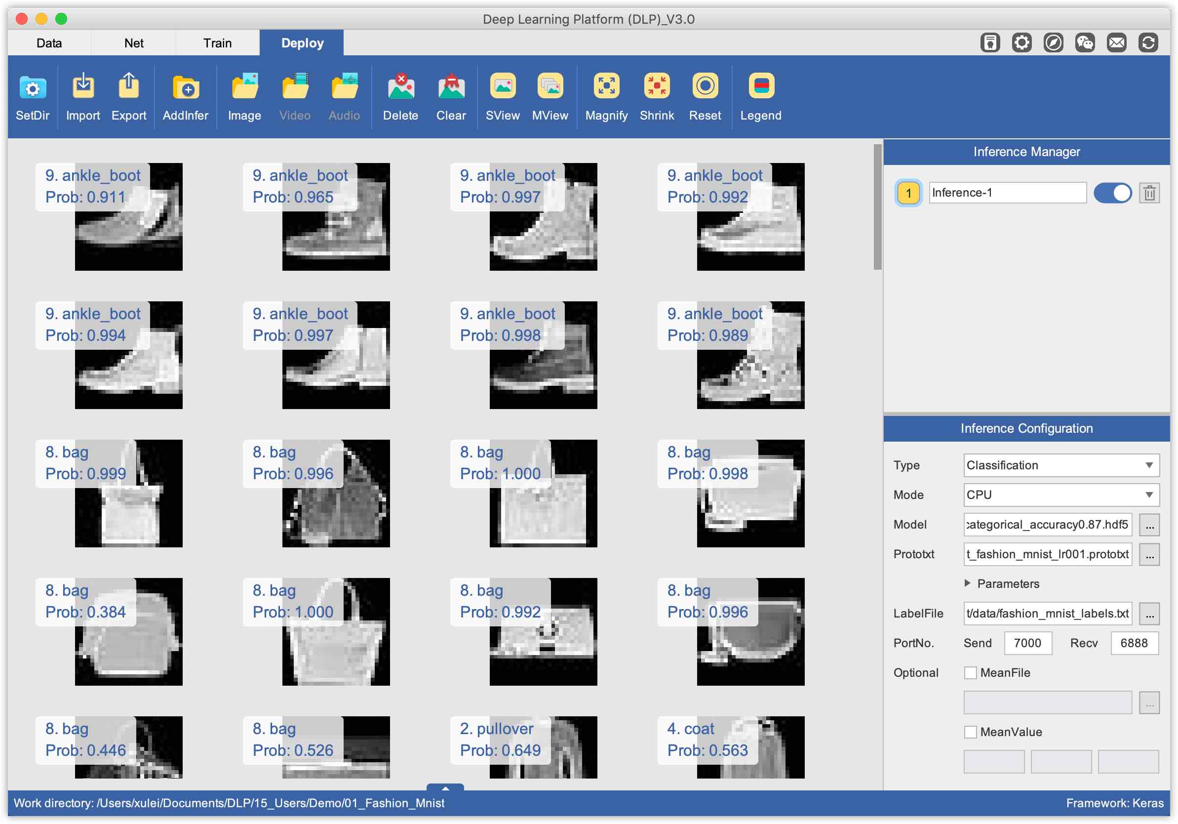
Once the engine is on, you can now do inference on unseen samples. You can either load a batch of images from a folder or load images one at a time. Let’s load a batch of images, specifically let’s evaluate our trained model on the test set of our dataset. To do so, click on the Image button on the top function panel and select the folder containing images of our test set. Once the images are loaded, the inference engine will start doing inference on each image and will return the predicted class label and the probability associated with it.

You can double click an image and see detailed predictions of top-5 probabilities.